
Empowering Valuation with Machine Learning: Tackling Complex Derivatives Classification

1. Overview of the Topic
1.1. Introduction
The market for structured products has experienced unprecedented growth in the post-Covid era. According to SRP data, the number of structured products issued in 2020 across EMEA and North America was approximately 60,000. This number increased to 266,000 in 2023 and to 327,000 in 2024. It is expected that this number will be exceeded again in 2025.
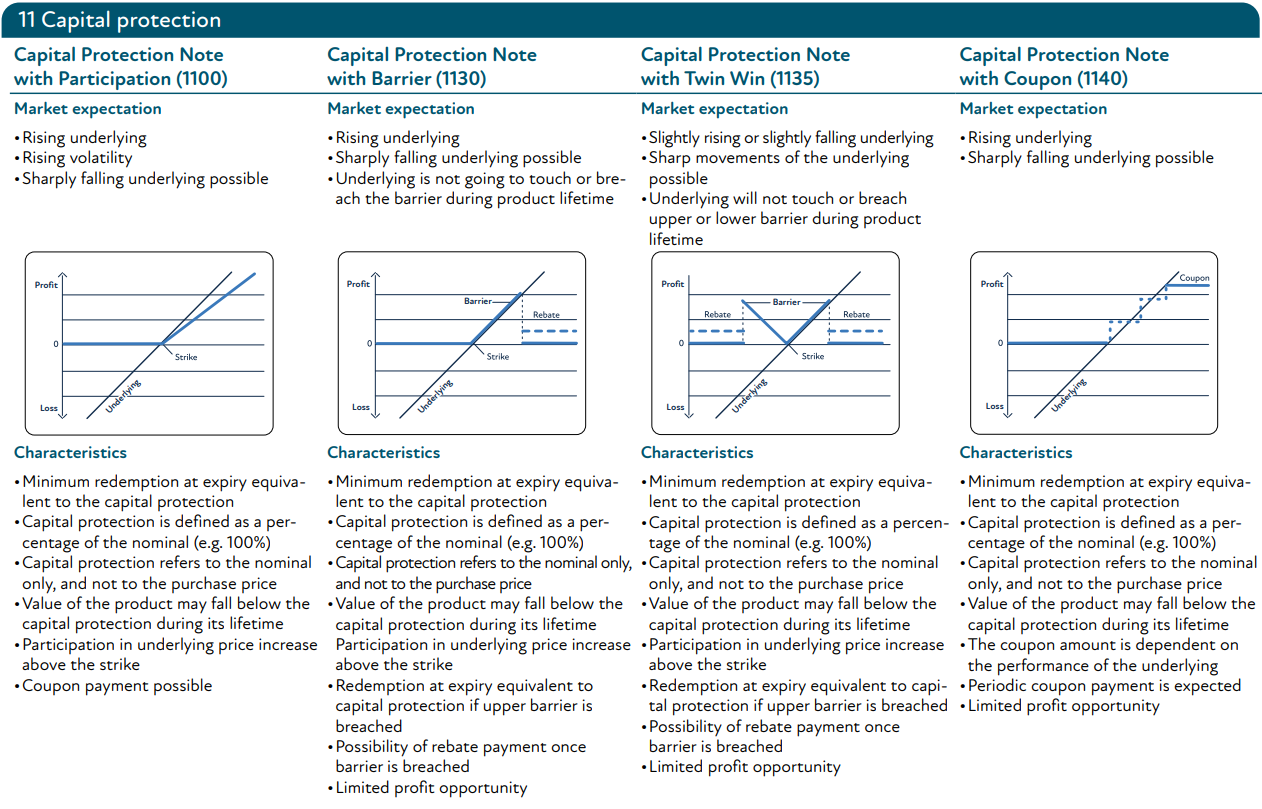
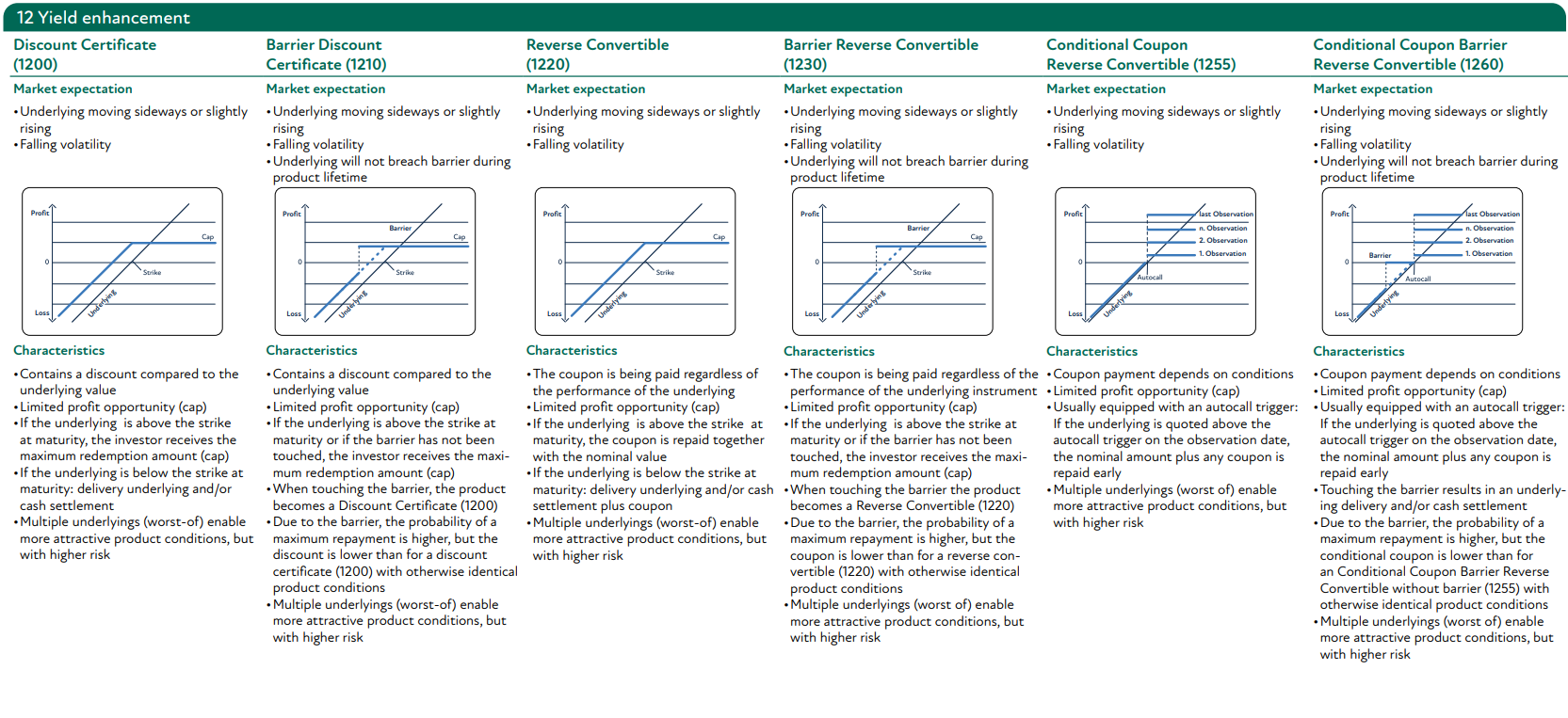
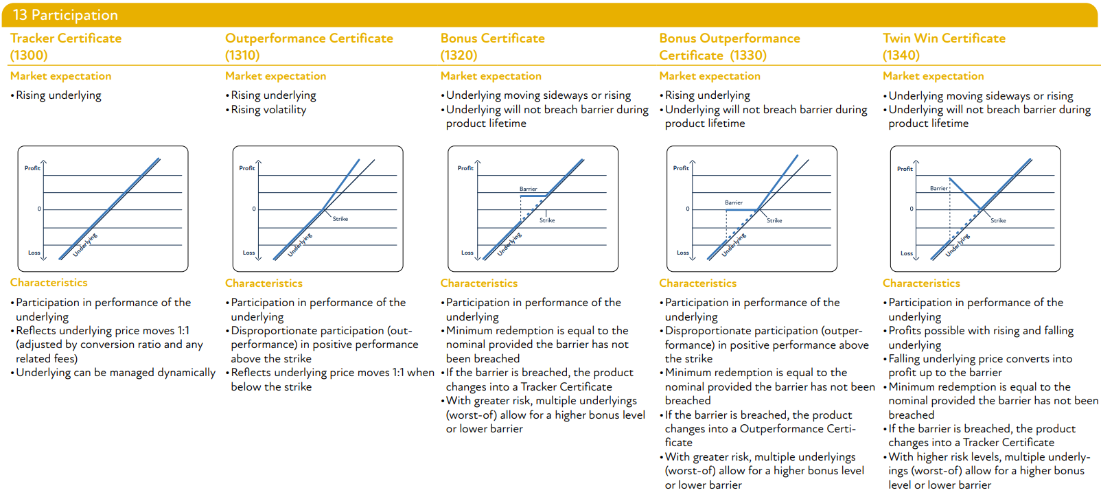
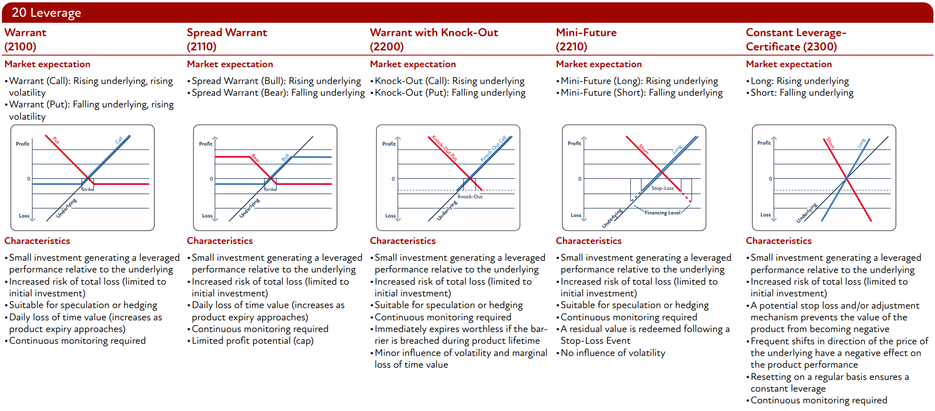
This market is inherently characterized by its immense diversity, offering tailor-made products to meet specific investor needs. Across asset classes, currencies, and issuers, this results in thousands of unique contracts. To navigate this complexity, coding schemes help with categorization. The Swiss Structured Products Association, for example, organizes instruments into broad clusters (see Appendix 5.1). However, the sheer variety within these clusters can create hundreds of nuanced sub-categories, complicating the process of distinguishing and pricing individual contracts.
Pricing these contracts accurately requires a detailed analysis of their termsheets—a task that is time-intensive and prone to human error. Accurate classification of structured products is critical for middle office and valuation teams to manage the operational and financial risks associated with these instruments. Proper categorisation ensures efficient trade capture, accurate risk reporting and streamlined lifecycle management. In addition, for valuation teams, detailed classifications enable accurate pricing methodologies tailored to the unique characteristics of each product.
At Finalyse, we handle the valuation of OTC derivatives and structured products, receiving hundreds of new instruments daily. This article highlights how we leverage machine learning to streamline this part of the valuation process, enabling accurate categorization without the need to read the termsheet. This approach has allowed us to handle large-scale valuations seamlessly, delivering rapid and precise results to our clients.
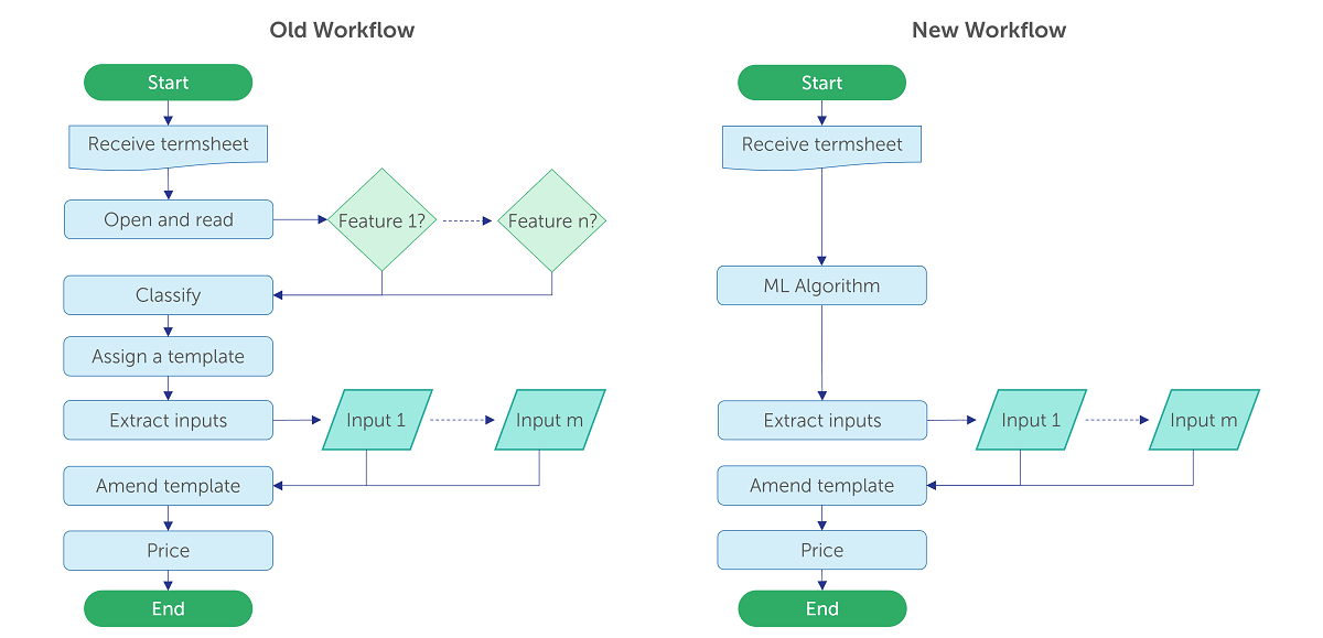
[figure 1]: Seamless pricing workflow chart
1.2. Goal and Requirements
The primary objective of this article is to demonstrate a robust text-based classification system capable of analyzing derivative termsheets to identify and categorize product types. Each classification must account for all relevant pricing-specific attributes. This process involves integrating termsheet data seamlessly into existing pricing tools and templates, ensuring accurate and tailored valuation.
The success of this system hinges on meeting the following criteria:
Accuracy: Predictions must achieve near-perfect accuracy to ensure valid pricing.
Flexibility: The model must generalize across diverse contract types and client-specific variations.
Speed: The process must integrate seamlessly into workflows, offering fast predictions even at scale.
These were the guiding principles during development.
The article will be structured as follows: A detailed methodology of the framework will be presented. Subsequently, the results will be discussed. Finally, we disclose a conclusion with recommendations for future applications.
2. Methodology
2.1. Problem Definition and Notation
For a given client, the classification problem can be formalized as follows:
- Let C = {c1, c2,…,cK} denote the set of K mutually exclusive classifications. Each ck ∈ C corresponds to a detailed derivative type.
- Let N = {n1, n2,…,nI} denote the set of I termsheets, where each ni ∈ N represents a single document.
- Let T = {t1, t2,…,tJ} denote the set of J terms across all termsheets, where each tj ∈ T is a distinct term within the set. For each termsheet ni, the terms Ti ⊆ T describe its content.
The goal of the algorithm is to classify a termsheet ni into one category ck based on the terms Ti. This is formalized as a mapping function f:
f (Ti) = ck
The following figure illustrates each step of the methodology:
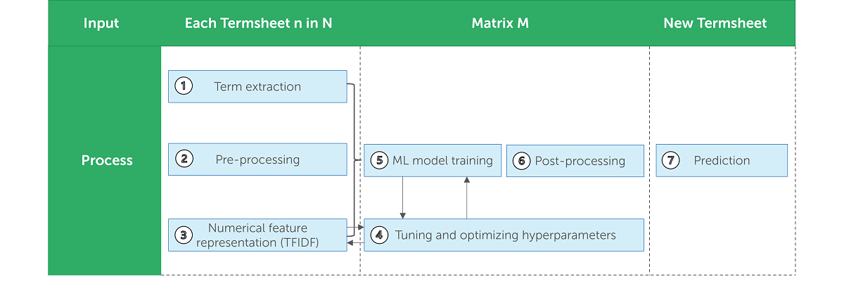
[figure 2]: Methodology
2.2. Data Pre-Processing
Effective pre-processing is essential to focus on relevant information and exclude extraneous content, such as branding, legal disclaimers, and other details that do not influence pricing. This stage systematically reduces noise, enhancing the algorithm's speed and accuracy.
For each termsheet ni, pre-processing reduces the set of terms Ti by approximately 50%, significantly improving the efficiency of both training and prediction. Since termsheets differ across clients, each requires tailored rules for extracting relevant text. A simple yet effective method is restricting extraction to specific page ranges or text spans defined by keywords. This works reliably as details critical to pricing are usually clustered together.
2.3. Numerical Feature Representation
With a clean set of terms Ti, each set needs to be converted to a numerical feature vector xi which quantifies the importance of each term in determining the particular product type. We employ the Term Frequency-Inverse Document Frequency (TFIDF) framework for this transformation, which is an NLP technique that measures the importance of each word in a sentence.
Given xi as the vector of feature importance for any set of terms Ti, define xij = TFIDF (tj, ni, Ti, N, I) as the numerical feature representation of any term tj ∈ Ti. This is computed as a product of two values:

2.3.1. Term Frequency (TF)
T F (tj,Ti) measures how frequently a term tj appears in one document ni, thereby quantifying its importance within that document:

with:

2.3.2. Inverse Document Frequency (IDF)
IDF (tj,ni,Ti,N,I) measures how important a term tjis in the whole set of documents N:

where:

Note the logarithm in the formula for IDF(tj,ni,Ti,N,I). It serves to diminish the importance of extremely common terms. If a term tj appears in all documents ni ∈ N, the logarithm ensures its IDF(tj,ni,Ti,N,I) weight is 0.
The output of the TFIDF process is a matrix M∈ RNxT, where each row corresponds to the numerical feature representation of all terms in T for a single termsheet ni, and each column represents the numerical feature representation of one term tj for all documents in N. Consequently, each xij refers to the TFIDF score of a term tj for termsheet ni:

The table below demonstrates a snippet of what M could look like in production:
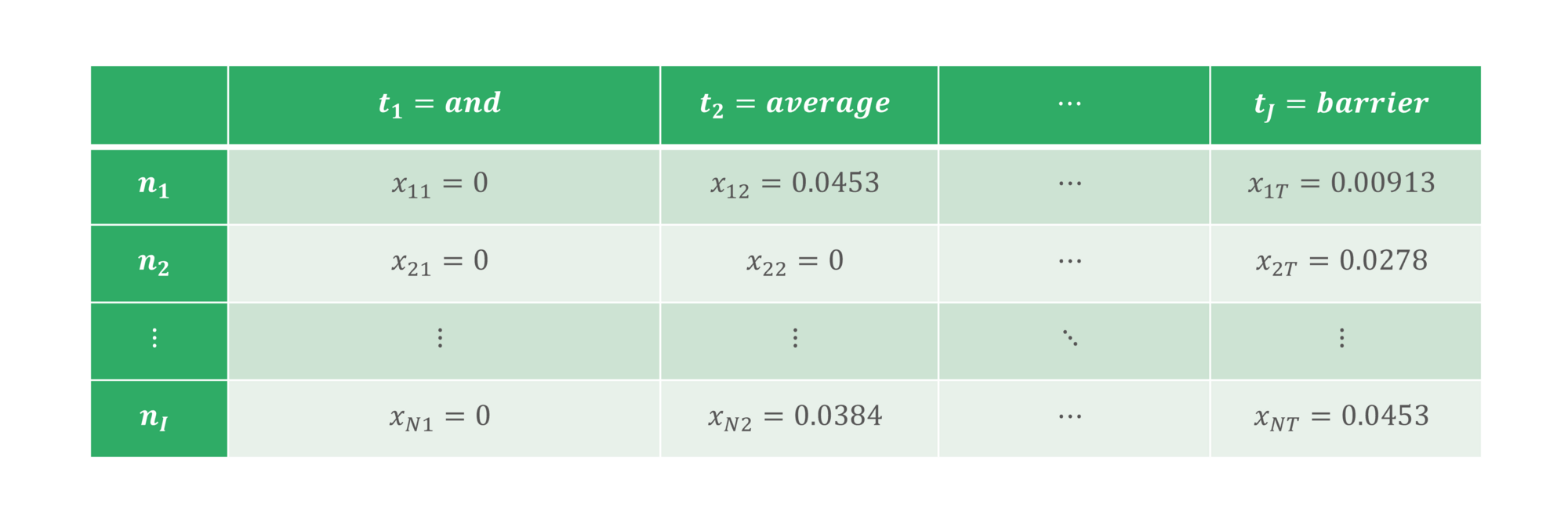
[figure 3]: TFIDF matrix M
2.4. Machine Learning Model
The chosen model for this task is Random Forest. While alternatives like XGBoost, Neural Networks, SVM, and Logistic Regression were explored, none matched Random Forest's balance of speed, accuracy, and reliability during hyperparameter tuning (see section 2.5). Hardware limitations restricted the complexity and accuracy of alternative models, confirming Random Forest as the optimal choice. Despite some base models achieving higher accuracy, Random Forest was favoured for its robustness against overfitting, ability to handle high-dimensional feature spaces, and effectiveness with diverse text features. The following sections detail the methodology, including input representation, model structure, training, and prediction phases.
2.4.1. Inputs and Notation
The problem is framed as a supervised classification task. Let the following inputs define the problem space:
- Let X = {x1, x2,…, xN} be a set of N numerical feature vectors derived from the set of termsheets ni ∈ N. Each xi is computed using the TFIDF representation of the terms Ti.
- Let Y = {y1, y2,…, yN} be a set of N corresponding classifications assigned to each termsheet ni, where each yi ∈ C.
The goal is to find a function f:X→Y, which maps the feature space X to the corresponding label set Y. Finding the optimal function f will then solve the mapping problem f(Ti)=ck.
2.4.2. Random Forest Structure
The Random Forest algorithm spans T decision trees:

where each tree ht(x) is a function mapping an input feature vector x ∈ X to a predicted instrument class ck ∈ C.
2.4.3. Training Procedure
Each decision tree ht (x) is trained on a bootstrap sample (Xt,Yt ) drawn with replacement from the original training dataset (X,Y). Let:

where xij ∈ X and yij ∈ Y.
At each step of tree construction, the algorithm decides how to split the data into subsets. A splitting criterion quantifies the "quality" of a potential split, guiding the algorithm toward decisions that improve the tree's predictive performance. For this, we have applied the popular Gini impurity defined as:

where pk is the proportion of data points in S that belong to class ck. At each node on the tree, a random subset of f features is selected from the total T dimensional feature space (f ≪ T). For each feature fj in the subset, the algorithm evaluates all possible threshold values t to compute the Gini impurity of the resulting splits. The feature fj* and threshold t* that minimize the weighted Gini impurity of the child nodes are chosen to split the data. The recursive splitting process continues until one of the stopping conditions is met (e.g. maximum tree depth, minimum number of samples in a node, etc.).
2.4.4. Prediction
Given a new termsheet ni ∉ N, we extract its set of terms Ti and represent them in numerical feature representation xi. Each decision tree ht in the trained forest generates a class prediction ht (xi) ∈ C for the input feature vector.
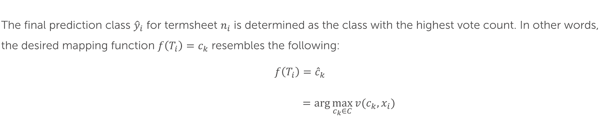
The Random Forest aggregates the predictions of all trees using majority voting. For each possible classification ck ∈ C, the vote count is computed as:

where:

2.5. Hyperparameter Tuning
Hyperparameter tuning optimizes model performance by balancing accuracy, computational efficiency, and generalization. Hyperparameters are the parameters of a machine learning model that are set before the training process begins, and include rules on data splitting and model flexibility. Tuning is used to select the best configuration of pre-defined hyperparameters that optimize the model’s performance for a specific task. Using tools like GridSearchCV, we systematically tune both the TFIDF vectorizer and Random Forest classifier.
TFIDF Vectorizer Tuning
The hyperparameters of the TFIDF Vectorizer directly influence the construction of the feature space, which affects both model training and final predictions. Examples include (among others):
- Document Frequency (max_df, min_df): Filters terms based on their frequency across documents to exclude common or rare terms.
- N-gram Range: Captures text units (e.g., unigrams, bigrams, trigrams) to enhance contextual understanding.
- Maximum Features: Limits the number of unique terms considered to decrease computational intensity.
Random Forest Tuning
Tuning the hyperparameters of the Random Forest classifier determines the trade-off between model flexibility and computational cost. Examples include (among others):
- Number of Trees: More trees reduce variance but increase training time.
- Maximum Depth: Controls overfitting by limiting tree complexity.
The combination of these parameters determines the flexibility of individual trees and the ensemble's overall strength.
2.5.1. Hyperparameter Optimization
Hyperparameter combinations are evaluated systematically using exhaustive cross-validation over a parameter grid. This tuning process ensures that both the feature representation and classification model are optimized for high accuracy and generalization across diverse termsheet types. By iteratively refining hyperparameters, the model adapts to the complexity of the dataset while maintaining computational efficiency.
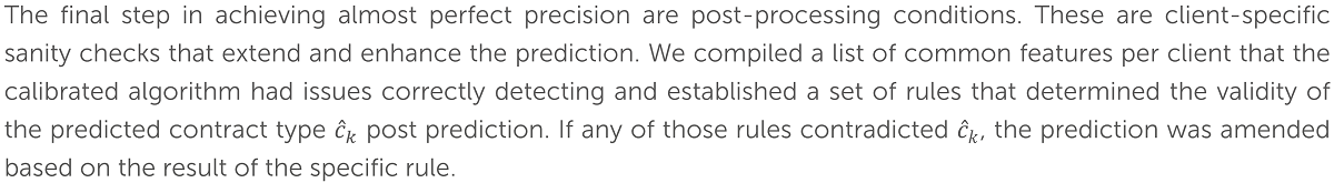
2.6. Data Post-Processing
3. Results
The implemented classification model was trained on a sample of I=1000 termsheets which spanned K=51 classification types.
The model achieves robust performance across all three critical criteria:
Accuracy
The initial out-of-sample accuracy of the Random Forest classifier reached 96%, measured as the proportion of correct predictions relative to the total number of predictions. Certain idiosyncratic nuances in client-specific termsheets initially posed challenges for achieving near-perfect accuracy. These were mitigated through the integration of post-processing rules tailored to individual clients, with which the accuracy consistently improved to exceed 99%.
Flexibility
The model demonstrates exceptional generalizability across diverse contract types and variations among clients. The TFIDF vectorization process captures patterns in textual features while excluding noise, making it adaptable to new termsheets and evolving contract structures. Additionally, hyperparameter tuning ensures that the model's underlying architecture balances its ability to learn complex patterns with its need to generalize effectively. The post-processing rules enhance this further by allowing the system to adapt dynamically to unique client-specific requirements and rare contract types.
Speed
Designed to integrate seamlessly into existing workflows, the model processes large volumes of termsheets efficiently. The computational efficiency of the Random Forest classifier and the optimization of hyperparameters ensure rapid predictions without compromising accuracy.
4. Conclusion
This article demonstrates the successful application of machine learning to the classification of OTC derivatives. By developing a robust pipeline—from data preprocessing and feature extraction using TFIDF, to classification with a Random Forest model with hyperparameter tuning and client-specific post-processing—the methodology achieves a high degree of accuracy over 99%.
Ultimately, this approach not only streamlines the valuation process but also enhances accuracy and efficiency, reducing the risk of human error. It highlights the transformative potential of machine learning in tackling financial challenges, setting a benchmark for automating and optimizing other similar workflows in the financial industry.
Applications of this methodology can be extended to domains beyond the financial industry and to any problem that requires text-based classification. Future analyses can push this framework further by exploring more sophisticated models like generative AI (for example LLMs) to improve accuracy if necessary, albeit with significantly higher hardware and computational demands.
5. Appendix
5.1. SSPA Product Classification (www.sspa.ch)