

Written by Long Le Hai, Consultant and Nemanja Djajic, Senior Consultant.
INTRODUCTION
As there is an ongoing progress in big data and machine learning, it is essential for credit scorecard models to adapt and effectively address the challenges of data preparation and feature engineering. An efficient feature engineering process in scorecard development can significantly improve the overall performance of credit scorecard models. This process typically involves data modification, data transformation, as well as dimensionality reduction part.
Apart from the traditional feature engineering techniques, that have been widely used for credit risk modelling, there are multiple novel techniques to pre-process data, solve data-quality issues and reduce the number of potential variables. In this blog post, we will explore alternative approaches that can be employed for variable transformation and feature engineering processes, by covering the following topics:
1. Missing Imputation
2. Variable Transformation Techniques
3. Dimensionality Reduction and Feature Selection
More detailed explanation for each of these topics is provided in the following sections.
1. Missing Imputation
Utilizing machine learning techniques for missing data imputation comes with its own set of advantages and disadvantages, much like any other approach. On the positive side, machine learning can capture complex patterns and relationships in the data, provide more flexibility and reduced bias. On the flip side, machine learning can potentially introduce data uncertainty and errors, overfitting or incur high computational costs. In this blog post, we will introduce three specific techniques for missing data imputation: k-Nearest Neighbour (kNN) Imputation, Random Forest Imputation, and Multiple Imputation by Chained Equations (MICE).
1.1 k-Nearest Neighbour (kNN) Imputation
k-Nearest Neighbour is non-parametric algorithm that relies on the concept of similarity measurement between data points. It is a distance-based imputation technique in which the process of kNN can be performed using various distance measures such as Euclidean or Manhattan distance.
In the presence of missing values, kNN imputation considers the available features of a data point and identifies the k closest neighbours based on their similarity. After that kNN calculates the similarity or distance between data points. By analysing the known values of these neighbouring data points, an approximation for the missing value can be estimated.
It is important to note that k (the number of nearest neighbours) is an important parameter. The value of ‘k’ determines the size of the neighbourhood around a data point. The optimal value of ‘k’ can be achieved by cross-validation. KNN can be more accurate than Mean Imputation, but It can be sensitive to outliers (distance-based algorithm) and computationally expensive.
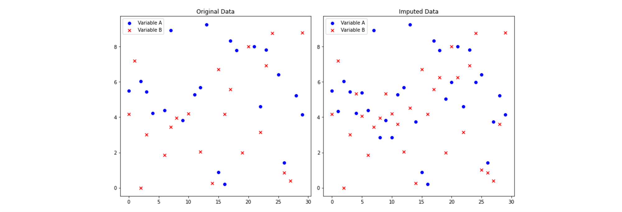
Below is a graphical representation of the k-Nearest Neighbours (kNN) algorithm's output for a small dataset with two variables. The dataset includes both original data with missing values and the imputed data after applying kNN imputation. This visualization allows us to compare the data distribution and assess the impact of imputation on the dataset:
1.2 missForest (Random Forest Imputation)
MissForest technique, as its name suggests, utilizes the Random Forest algorithm for imputing missing values. This algorithm is often referred to as regression imputation since it leverages information from other variables to predict the missing values in a variable by using regression models. In other words, missForest builds multiple regression models to predict the missing variable using other variables as the predictors. The predicted values will be the imputed values in each iteration of missForest algorithm.
MissForest leverages the power of random forests to capture complex relationships and patterns in the data to impute missing values. Through iteratively predicting missing values for each variable, it takes into account the dependencies between variables, potentially resulting in improved imputation accuracy when compared to simple imputation methods.
MissForest is particularly useful when dealing with mixed types of datasets that contain both numerical and categorical variables. It is also robust to noisy data because of its built-in feature selection. However, missForest can be extremely computationally demanding and can cause memory errors.
1.3 Multiple Imputation by Chained Equations (MICE)
Similar to previous method, Multiple Imputation by Chained Equations (MICE) is a parametric imputation method that involves iteratively imputing missing values for each variable using regression models. It is a widely used technique in various fields, including credit risk modelling, for improving data analysis by reducing bias and enhancing parameter estimate accuracy. MICE is known for its flexibility in handling missing data in both categorical and continuous variables.
The computation approach of MICE involves several key steps. First, it initializes the missing values with reasonable estimates or imputations. Then, it iteratively cycles through each variable with missing data, treating it as the dependent variable and using the other observed variables as predictors. At each iteration, it creates a regression model, imputes missing values, and repeats this process multiple times to obtain a set of imputed datasets. This generates multiple imputed datasets to account for the uncertainty associated with missing data. After all iterations are completed, the final results are combined to produce valid parameter estimates and standard errors. MICE's strength lies in its adaptability to various types of data and its ability to provide robust imputations for more accurate and reliable statistical analysis. In the development of credit scoring models, the technique of MICE is very useful, especially for addressing missing data problems caused by data quality (DQ) issues.
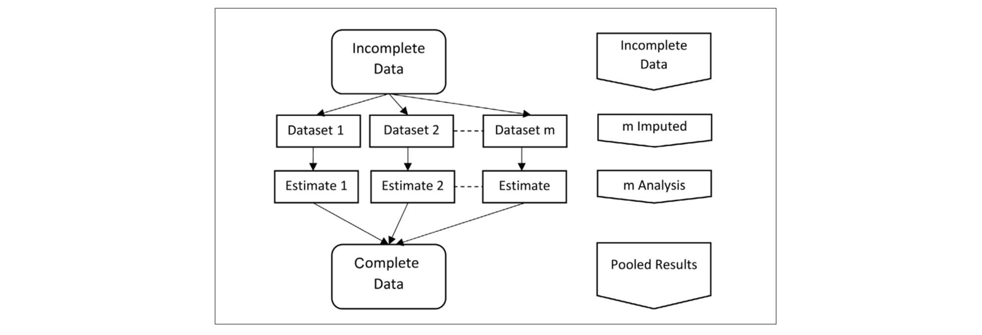
Source: Alruhaymi, A. and Kim, C. (2021) Why Can Multiple Imputations and How (MICE) Algorithm Work?
2. Variable Transformation
Many statistical and machine learning algorithms assume that all numerical variables should follow Normal distribution (data may not strictly follow Normal distribution but at least it should have Normal-like distribution shape). To address those issues related to nonlinearity, heteroscedasticity, or skewness in the data, we use various variable transformation techniques in our work. Power transformation methods such as Box-Cox and Yeo-Johnson offer automated approaches to reshape variables into a more Normal-like distribution. Those techniques usually improve performance and interpretability of machine learning models, normalize data, and stabilize variance.
Apart from those advanced methods, traditional variable transformation methods that are commonly used for adjusting numerical data (or for converting categorical variables into numerical format) are WoE transformation and encoding techniques.
2.1 Weight-of-Evidence Transformation
WoE method transforms continuous predictors into bins to represent the strength of the relationship between a selected feature and target variable. It replaces the original feature values with their corresponding WoE values. Moreover, WoE can be conveniently converted into Information Value values to assess the significance of predictors and supports the selection of a subset of useful variables.
There are some benefits of WoE in scorecard development, namely:
- Reducing the effect of outliers
- Missing values treatment (missing values represent separate bin).
- Variable transformation (convert continuous predictors to categorical predictors)
Nevertheless, it is important to acknowledge that while WoE shows robustness to outliers and missing values it does not entirely eliminate their influence. As a result, incorporating additional machine learning-based feature engineering techniques can prove advantageous in addressing the limitations of WoE.
2.2 Box-Cox Transformation
The key idea behind the Box-Cox transformation is to find the optimal value of the power parameter, lambda (λ), that maximizes the normality of the transformed variable. By varying λ, the Box-Cox transformation can handle a wide range of data distributions, from highly skewed to symmetric. This flexibility makes it particularly useful in situations where the data does not conform to the assumptions of linear regression models, such as heteroscedasticity or nonlinearity. The optimal value of λ can be estimated using maximum likelihood estimation. Box-Cox transformation assumes input variables are strictly positive.
2.3 Yeo-Johnson Transformation
Similar to the Box-Cox, the Yeo-Johnson aims to find the optimal value of the power parameter, lambda (λ), to achieve a more normal distribution of the transformed variable. However, unlike the Box-Cox transformation, the Yeo-Johnson transformation supports both positive and negative values of lambda, allowing it to handle a broader range of data distributions (including those with zero and negative values). The optimal value of λ in the Yeo-Johnson transformation can be estimated using numerical optimization techniques.
2.4 Robust Scaling
It is important to remove outliers for continuous variables before fitting the model to bring the individual variables into the same scale. If some variables are significantly larger or smaller in comparison to others, these variables can dominate or scale the learning algorithms.
Winsorization is a well-popular technique to deal with outliers of continuous variables in credit risk models. Winsorization handles outliers by capping the extreme values. As a result, winsorization will cause the information loss due to capping the values, and the efficiency of winsorization is heavily dependent on threshold selections. Robust scaling is an alternative approach to handle outliers with some clear advantages relative to winsorization.
Robust scaling is used to standardize or rescale data in a way that is robust to the presence of outliers. Robust Scaling subtracts each data point to the median and then divides by the difference between 75th percentiles and 25th percentiles. Thus, this scaling method is more robust to the outliers and less sensitive to the extreme values. Moreover, Robust scaling does not cause the information loss because it does not cap or remove the data points.
2.5 One-Hot Encoding
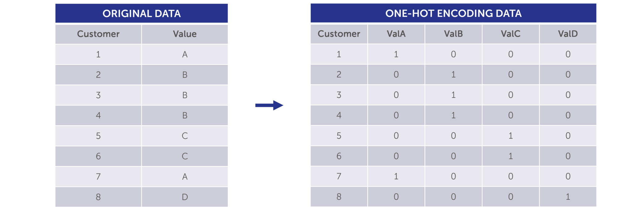
One-hot encoding is a technique used to convert categorical data into a binary format that machine learning/or traditional modelling algorithms can understand. It creates a binary column (or "dummy variable") for each unique category, assigning a 1 to the column corresponding to the category of the data and 0s to all others. This method is effective for handling categorical features in machine learning and is valuable when there is no inherent order or relationship between the categories.
2.6 Dummy Encoding
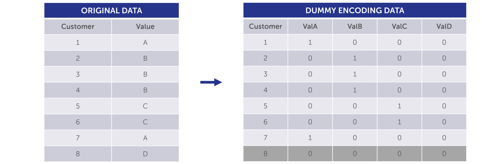
Just like one-hot encoding, dummy encoding transforms categorical data into a numerical format. However, it differs in that it excludes one category as a reference, preventing multicollinearity, and using "0" and "1" to represent the remaining categories.
3. Dimensionality Reduction and Feature Selection
Dimensionality reduction is an approach employed to reduce the number of features (variables) in a dataset. While it effectively transforms a high-dimensional set of variables into a lower-dimensional representation, it strives to preserve as much information as the original dataset. In credit risk models, where numerous variables are typically available, effectively selecting the optimal subset of predictors helps model to perform better. Furthermore, dimensionality reduction aims in mitigating the "curse of dimensionality".
3.1 Principle Component Analysis (PCA)
Principal Component Analysis (PCA) is a powerful technique employed in credit risk analysis to mitigate the challenges posed by high-dimensional data. In the realm of dimensionality reduction, PCA assists in reducing the complexity of credit risk models by transforming the original set of correlated variables into a smaller set of uncorrelated variables known as principal components. By selecting a subset of these components that explain a significant portion of the variance in the data, PCA enables a more efficient representation of the credit risk information.
Consequently, PCA aids in identifying the key underlying factors that drive credit risk, enabling financial institutions to make informed decisions, assess portfolio diversification, and optimize risk management strategies. By effectively condensing the dimensionality of credit risk data, PCA enhances the accuracy and computational efficiency of credit risk models, ultimately contributing to more robust credit risk assessments and improved overall risk management practices.
In credit risk models, PCA is particularly useful for variable clustering. Instead of reducing the dimensionality of the dataset, PCA is used to identify patterns of correlation or clustering among the original features in high-dimensional data. The primary goal of variable clustering is to identify groups of features that exhibit similar patterns of variation to reduce the dimensionality of the dataset and to map relationships among variables, making it easier to select a subset of relevant features for model fitting step. In contrast to data point clustering using PCA, where the central objective is to group individual data point based on their data profiles, variable clustering focuses on identifying relationships among features and reducing feature dimensionality.
3.2 Linear discriminant analysis (LDA)
While PCA falls under the category of unsupervised learning when it comes to dimensionality reduction, LDA, on the other hand, belongs to the realm of supervised learning. LDA is more effective than PCA in classification dataset because LDA focuses on maximizing class separability while finding the linear combination of the predictors in a lower dimensional space. In Probability of Default models, we need to deal with class separability which means that we try to keep class of “Good” and class of “Bad” (based on Definition of Default) as far as possible but try to maintain the minimum separation between data points within the same class. This makes LDA particularly valuable in feature engineering steps to reduce dimensionalities in credit risk models before modelling step to improve the performance of both binary and multi-class classification problems.
3.3 T-SNE (T-distributed Stochastic Neighbour Embedding)
T-SNE is non-linear dimensionality reduction which is applicable to separate data that cannot be separated by a straight line. Also, t-SNE is a powerful visualization tool to explore high-dimensional data with unsupervised learning algorithm. T-SNE can map higher-dimensional features into two- or three-dimensional space so that we can observe the data through the plot. This ability of t-SNE is valuable to deal with the dataset which has pattern that cannot easily map or separate by linear relationship. T-SNE leverages stochastic characteristic to maintain probability distribution of original data similar to lower dimensional space.
Unlike PCA which is linear and deterministic, t-SNE is non-linear and randomized. PCA focuses on retaining the variance present in the data, while t-SNE emphasizes the preservation of relationships among data points within a lower-dimensional space. T-SNE outperforms PCA in scenarios when preserving local structure, capturing nonlinear relationships, and visualizing complex patterns. However, PCA is more computationally efficient, and PCA usually performs better than t-SNE in smaller dataset.
CONCLUSION
In conclusion, the utilization of machine learning (ML) techniques in feature engineering for credit models has proven to be a pivotal advancement in credit risk modelling. The machine learning-based feature engineering techniques have demonstrated their value in improving the accuracy, interpretability, and generalization of credit models. Moreover, these methods provide the flexibility to adapt to changing business requirements and the robustness to risk thresholds. From a regulatory perspective, it's worth noting that while ML may not be widely accepted as the primary methodology for constructing credit models, incorporating ML techniques into the feature engineering step can be a valuable addition, especially in the context of credit model development. As both AI world and financial industry continues to evolve, the integration of these techniques is essential for staying ahead of the curve.